Riemannian Geometry Background

Note, this post is a work-in-progress. I aim to recreate a shortened version of the background section from my dissertation “Generalizing Regularization of Neural Networks to Correlated Parameter Spaces” as a blog post

Given a real, smooth manifold \(M\), at each point $p \in M$ we define a vector space $T_pM$ called the tangent space of $M$ at p. The tangent space is a flat plane consisting of all tangent vectors to the manifold at the point $p$. The dimension of the tangent space at every point of a connected manifold is the same as that of the manifold itself [Carmo 1992]. An example of the tangent space at a point on a 2-dimensional manifold embedded in 3-dimensional space is shown in the figure below. A Riemannian metric $g$ assigns to each $p \in M$ a positive-definite inner product over the tangent space $g_p: T_pM \times T_pM \rightarrow \mathbb{R}$. The metric, thus, assigns a positive value to every non-zero tangent vector [Dodson and Poston 2013]. A real, smooth manifold $M$ with a Riemannian metric $g$ is a Riemannian manifold denoted as $(M,g)$. The most familiar example of a Riemannian manifold is Euclidean space. Let $y^1, …, y^n$ denote the Cartesian coordinates on $\mathbb{R}^n$. Then the metric tensor is $g_p = \mathbf{I} \in \mathbb{R}_+^{n \times n}$ and the inner-product is the familiar definition of the dot-product for Euclidean geometry $\sqrt{g_p(\mathbf{u},\mathbf{v})} = \sqrt{\mathbf{u}^T\mathbf{I}\mathbf{v}} = \sqrt{\sum_i u_i v_i}$. For $\mathbb{R}^2$ this results in the traditional Pythagorean theorem. Thus, the metric generalizes the calculation of distance to non-Euclidean spaces and to arbitrary dimensions. The identity matrix is also called the canonical Euclidean metric.

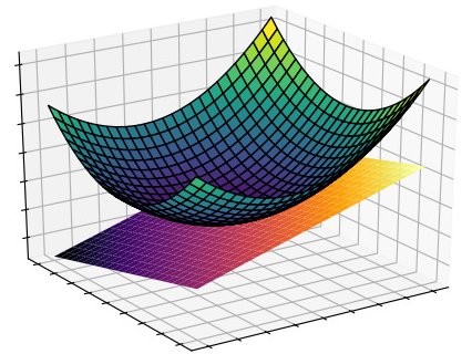
Figure 1: Example of the Tangent Space (orange shades) at a point on a 2-dimensionalmanifold (green shades).

This inner product can be | used to define a norm for tangent vectors $|\cdot|_p:T_pM \rightarrow \mathbb{R}$ by $|\mathbf{v}|_p = \sqrt{g_p(\mathbf{v},\mathbf{v})}$, as well as other geometric notions such as angles between vectors and the local volume of the manifold [Carmo 1992; Amari 2016]. The local volume of a manifold is defined as the determinant of the metric tensor and used in the Jeffreys prior to make it invariant to a change of coordinates. For example we can look at the $UV$ coordinate system where $UV \subseteq \mathbb{R}^2$. Let $\mathbf{a} = a_1 \frac{\partial}{\partial u} + a_2 \frac{\partial}{\partial v}$ and $\mathbf{b} = b_1 \frac{\partial}{\partial u} + b_2 \frac{\partial}{\partial v}$ where $\frac{\partial}{\partial u}, \frac{\partial}{\partial v}$ are the basis vectors of some tangent space and $a_1, a_2, b_1, b_2 \in \mathbb{R}$. Then, using the bilinearity of the dot product: $\mathbf{a} \cdot \mathbf{b}$
$= a_1 b_1 \frac{\partial}{\partial u} \cdot \frac{\partial}{\partial u} + a_1 b_2 \frac{\partial}{\partial u} \cdot \frac{\partial}{\partial v} + a_2 b_1 \frac{\partial}{\partial u} \cdot \frac{\partial}{\partial v} + a_2 b_2 \frac{\partial}{\partial v} \cdot \frac{\partial}{\partial v}$
$=$ \(\begin{bmatrix} a_1 & a_2 \end{bmatrix}\) \(\begin{bmatrix} \frac{\partial}{\partial u} \cdot \frac{\partial}{\partial u} & \frac{\partial}{\partial u} \cdot \frac{\partial}{\partial v} \\ \frac{\partial}{\partial u} \cdot \frac{\partial}{\partial v} & \frac{\partial}{\partial v} \cdot \frac{\partial}{\partial v} \end{bmatrix}\) \(\begin{bmatrix} b_1 \\ b_2 \end{bmatrix}\) In this case the metric tensor is \(g = \begin{bmatrix} \frac{\partial}{\partial u} \cdot \frac{\partial}{\partial u} & \frac{\partial}{\partial u} \cdot \frac{\partial}{\partial v} \\ \frac{\partial}{\partial u} \cdot \frac{\partial}{\partial v} & \frac{\partial}{\partial v} \cdot \frac{\partial}{\partial v} \end{bmatrix}\), \(\mathbf{a} \cdot \mathbf{b} = g(\mathbf{a}, \mathbf{b})\), the norm of a tangent vector is $|\mathbf{a}| = \sqrt{g(\mathbf{a}, \mathbf{a})}$ and the angle \(\theta\) between two tangent vectors is $cos(\theta) = \frac{g(\mathbf{a}, \mathbf{b})}{|\mathbf{a}||\mathbf{b}|}$.

When $\begin{bmatrix} a_1 & a_2 \end{bmatrix} = \begin{bmatrix} b_1 & b_2 \end{bmatrix} = \begin{bmatrix} du & dv \end{bmatrix}$ then the inner-product describes the instantaneous change along the tangent space: \(ds^2 = \begin{bmatrix} du & dv \end{bmatrix} \begin{bmatrix} \frac{\partial}{\partial u} \cdot \frac{\partial}{\partial u} & \frac{\partial}{\partial u} \cdot \frac{\partial}{\partial v} \\ \frac{\partial}{\partial u} \cdot \frac{\partial}{\partial v} & \frac{\partial}{\partial v} \cdot \frac{\partial}{\partial v} \end{bmatrix} \begin{bmatrix} du \\ dv \end{bmatrix}\)

We also note that by the chain rule \(\begin{bmatrix} du \\ dv \end{bmatrix} = \begin{bmatrix} \frac{\partial u}{\partial x} & \frac{\partial u }{\partial y} \\ \frac{\partial v}{\partial x} & \frac{\partial v}{\partial y} \end{bmatrix} \begin{bmatrix} dx \\ dy \end{bmatrix}\) where $dx$ and $dy$ are changes in the $XY$ coordinate system. Thus: $ds^2$
\(= \begin{bmatrix} du & dv \end{bmatrix} \begin{bmatrix} \frac{\partial}{\partial u} \cdot \frac{\partial}{\partial u} & \frac{\partial}{\partial u} \cdot \frac{\partial}{\partial v} \\ \frac{\partial}{\partial u} \cdot \frac{\partial}{\partial v} & \frac{\partial}{\partial v} \cdot \frac{\partial}{\partial v} \end{bmatrix} \begin{bmatrix} du \\ dv \end{bmatrix}\)
\(= \begin{bmatrix} dx & dy \end{bmatrix} \begin{bmatrix} \frac{\partial u}{\partial x} & \frac{\partial u }{\partial y} \\ \frac{\partial v}{\partial x} & \frac{\partial v}{\partial y} \end{bmatrix}^T \begin{bmatrix} \frac{\partial}{\partial u} \cdot \frac{\partial}{\partial u} & \frac{\partial}{\partial u} \cdot \frac{\partial}{\partial v} \\ \frac{\partial}{\partial u} \cdot \frac{\partial}{\partial v} & \frac{\partial}{\partial v} \cdot \frac{\partial}{\partial v} \end{bmatrix} \begin{bmatrix} \frac{\partial u}{\partial x} & \frac{\partial u }{\partial y} \\ \frac{\partial v}{\partial x} & \frac{\partial v}{\partial y} \end{bmatrix} \begin{bmatrix} dx \\ dy \end{bmatrix}\)
= \(\begin{bmatrix} dx & dy \end{bmatrix} \begin{bmatrix} \frac{\partial}{\partial x} \cdot \frac{\partial}{\partial x} & \frac{\partial}{\partial x} \cdot \frac{\partial}{\partial y} \\ \frac{\partial}{\partial x} \cdot \frac{\partial}{\partial y} & \frac{\partial}{\partial y} \cdot \frac{\partial}{\partial y} \end{bmatrix} \begin{bmatrix} dx \\ dy \end{bmatrix} = (ds')^2\).
This reflects two important points. Firstly that the distance calculation with the metric tensor is invariant under a change of coordinate systems. Secondly that the metric tensor transforms using the Jacobian matrix $\mathbf{J_f}$, the matrix of all first-order partial derivatives of a function $\mathbf{f}: XY \rightarrow UV$ that maps between coordinate spaces. Thus $g’ = \mathbf{J_f}^T g \mathbf{J_f}$ where $g’$ is the metric tensor in the $XY$ coordinate system and is known as the pullback metric of $g$ (for $UV$ space) from $\mathbf{f}$. The invariance of the metric tensor to a change of coordinates allows us to compute the inner product of tangent vectors in a manner independent of the parametric description of the manifold and so we can define a notion of distance in the $UV$ space but calculate the distance in the $XY$ coordinate system.

We have described the relationship between a manifold, its metric tensor and tangent bundle (set of all tangent spaces on the manifold), as well as how to map between different coordinate spaces. The final step is to describe how to obtain a metric tensor to begin with. Regions of a manifold are described using charts, where one or more charts are combined to form an atlas [Jost 2008; Gauld 1974]. A chart for a Riemannian manifold $(M,g)$ is a diffeomorphism $\varphi$ from an open subset $U \subset M$ to an open subset of a Euclidean space. The chart is denoted as the ordered pair $(U,\varphi)$. Since charts map onto Euclidean space we can then use the canonical Euclidean metric and also transform the points on the manifold to points in this Euclidean space where we can calculate distance. However if we wish to still work in the original space with the defined notion of distance in Euclidean space, we may then pullback the metric from the Euclidean space using the locally defined chart to obtain a metric tensor for the tangent space of the manifold. It is important to note that the pullback metric is not necessarily positive definite and so the manifold described by the pullback metric may not be Riemannian, but rather pseudo-Riemannian [Jost 2008]. Pseudo-Riemannian manifolds are a generalization of Riemannian manifolds where the positive definite constraint on the metric tensor is relaxed such that the metric tensor is only required to be everywhere non-degenerate. The non-degenerate property means that there is no non-zero $\mathbf{X} \in T_pM$ such that $g_p(\mathbf{X},\mathbf{Y}) = 0$ for all $\mathbf{Y} \in T_pM$. This is in contrast to the positive-definite constraint where for a non-zero $\mathbf{X} \in T_pM$ then $g(\mathbf{X}, \mathbf{Y}) \neq 0$ for all $\mathbf{Y} \in T_pM$.

Specifically for the case of NNs, we note that the parameter space of a probabilistic model forms a statistical manifold and by extension a Riemannian manifold [Rao 1945]. The metric tensor for statistical manifolds is the Fisher Information Matrix [Skovgaard 1984; Amari2016] shown earlier in Equation \ref{eq:Fisher}. If we interpret the loss function as a coordinate chart from the $N$-dimensional parameter space onto the $1$-dimensional Euclidean space then the Fisher Information Matrix is viewed as the pullback metric of the canonical Euclidean metric from the expected value of the loss. To show this we make use of the fact that since the loss is 1-dimensional then $L = \theta^TJ_L$ which is the usual notion of the differential of $L$. Hence: $E_\mathbf{X}[L^2] = E_\mathbf{X}[\theta^TJ_LJ_L^T\theta] = \theta^TE_\mathbf{X}[J_LJ_L^T]\theta = \theta^TI(\theta)\theta$.

The equality of the Fisher Information Matrix and Hessian matrix is also significant as the Hessian is used in the area of a critical point on a Riemannian manifold to obtain the principal curvatures [Porteous 2001], and as a result the shape operator at that point [Spivak1970]. In the case of a Riemannian manifold the shape operator is defined as the determinant of the Hessian matrix $det(H(\theta))$ [Koenderink and Van Doorn 1992]. The principal curvatures are defined as the eigenvectors of the Hessian matrix and decompose the manifold into orthogonal dimensions of curvature, with the first eigenvector reflecting the dimension of most curvature. The eigenvalues from the eigen-decomposition of the Hessian is known as the spectrum of the Hessian and the determinant of the Hessian can be calculated from the product of its eigenvalues. The Fisher Information Matrix (and by extension Hessian) is also significant as it upper-bounds the inverse covariance matrix of the parameters of a statistical model through the Cram'er-Rao Lower bound which states that $\Sigma^{-1} \leqslant I(\theta)$. As a result larger elements of the Fisher Information Matrix reflect that there is a lower degree of variance in the model parameters and more certainty that those parameters are necessary for fitting the training data. As stated in Chapter \ref{Intro} we believe this to be useful information for creating a regularizer by using the Riemannian distance to restrict the parameters of an NN. In light of this the Metric regularizer can be viewed as regularizing the low variance parameters of an NN more strictly, while the more irrelevant and high variance parameters are regularized less.

The Hessian matrix also provides the link between Riemannian Geometry and previous work with NNs as there has been a significant amount of work exploring the Hessian of the loss function in recent years. Most of these works have centered around the eigen-decomposition of the Hessian and the impact of flat regions of the landscape on both first and second-order training methods. Examples include the observation that the spectrum of the Hessian contains a few, large Eigenvalues but the large majority of Eigenvalues are near zero [Sagunetal.2017]. It was also observed that various changes to the hyper-parameters during training change the final parametrization learned by the model, but that these minima tended to lie along the same connected basin in the loss landscape. This was extended by y Gur-Ariet al.[2018] which empirically studied the overlap of the direction followed by GD and the directions corresponding to the large (top) Eigenvalues of the Hessian. It was found that after a brief warm-up period GD tended to follow these top directions nearly exclusively. There has also been work that aims to utilize the second-order information to create new practical algorithms that are more suited to optimizing non-convex manifolds. In Dauphinet al.[2014] the gradients of normal GD update steps are multiplied by the inverse of the absolute values of the Hessian matrix as well as the top Lanczos vectors of the Hessian. This creates an update step that is well adapted to escape saddle points within the loss landscape but is still able to effectively optimize the manifold.

A common consideration of all previous work regarding the Hessian is that the loss landscape contains flat regions along which the parameters of the network can be changed without affecting the network’s loss. This results in the Hessian matrix being singular. These flat regions are a result of covariant parameters that may be changed in a coordinated manner without changing the function approximation of the network. Such covariant parameters naturally occur with the addition of hidden layers to the model, resulting in parameters along the same path through the network becoming correlated. In addition the increase in width of the layers results in neurons of the same layer learning similar mappings and becoming interchangeable. While flat regions of the loss landscape reflect that the training loss is not affected by a change in parameter values along the flat path, different parametrizations may have significantly different performance on unseen data. This is because many network parametrizations can perfectly fit the seen data (data sampled from the data subspace) but perform different function approximations for unseen data (over the data null-space). The effective handling of the data null space is the point of regularization as it constrains the function approximation for unseen data. By creating a bias for the model parameters towards $0$ we constrain the model to simpler function approximations that interpolate smoothly between the seen data points. The necessity of regularization for data-constrained problems can be seen from Bayes’ rule where a prior is needed for data-constrained Bayesian inference. As the quantity of data increases ($P \rightarrow \infty$) the MAP solution converges to the ML solution, reflecting the decreasing need for the prior/regularization.